Flux-Corrected Transport

Flux-Corrected Transport (FCT) is a conservative, monotone technique
for integrating generalized continuity and hydromagnetic equations. It
is especially useful for solving compressible-flow problems,
particularly those involving shock and rarefaction waves, and contact
discontinuities. FCT accomplishes this objective by combining
integration schemes with low and high orders of spatial accuracy. The
low-order scheme provides a monotone solution, usually by the
introduction of diffusive numerical fluxes, while the high-order
scheme provides high accuracy in regions of smooth flow and shallow
gradients. The high-order solution is obtained by "antidiffusing" the
low-order, monotone solution, but only to such an extent that no new
extrema are created and no existing extrema are accentuated. This is
done by limiting, or "correcting," the antidiffusive fluxes of the
high-order scheme, hence the name Flux-Corrected Transport.
FCT was the first of the class of high-order, monotone schemes (FCT is
one of many schemes that can be classified TVD) for solving
generalized continuity equations (e.g., the equations of Eulerian
hydrodynamics). The version of FCT that was used for all of the
computations displayed at this site was originally coded by the
Laboratory for Computational Physics at the Naval Research Laboratory.
Click here to get the code.
Click on the pictures below to see
some typical results that I have obtained for both reactive and
non-reactive flow problems.
Shock wave diffraction
The set of pictures show a Mach 2.44 shock wave diffracting around a
45 degree wedge. (This problem was a benchmark problem used by the
CFD Society of Canada for their 1994 conference).
500 (horizontal) 380 (vertical) computational cells
Click on smaller images to see larger ones
|
Time:
|
60 microseconds
|
87 microseconds
|
|
|

(JPEG, 33 KB)
|
(JPEG, 64 KB)
|
1000 (horizontal) by 720 (vertical) computational cells
Click on small images to see larger ones
|
Time:
|
60 microseconds
|
87 microseconds
|
|
Regular Grid:
|
(JPEG, 40 KB)
|
(JPEG, 79 KB)
|
|
Jiggled Grid:
|
(JPEG, 34 KB)
|
(JPEG, 66 KB)
|
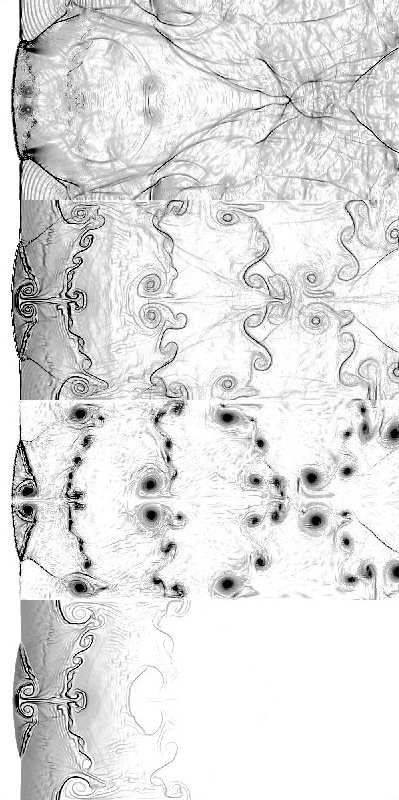
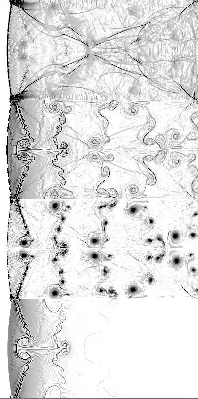
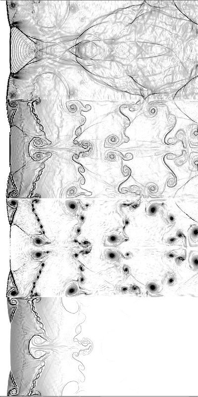
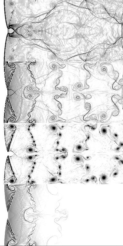
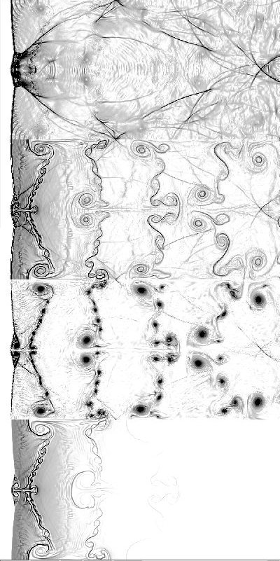
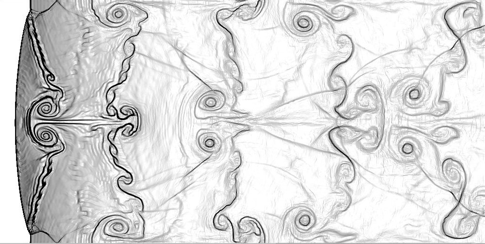
Detonations
The following results were obtained using a direction split FCT code
with single step chemistry and Arrhenius kinetics. The pictures are
plots of (from top to bottom) pressure gradient, temperature gradient,
vorticity, and gradient of fuel mass fraction. The pictures obtained
for overdrive 1.2, activation temperature 10 and heat release
parameter 50. They are smoother than other results
because in these computations, grid jiggling was used on the 1000 by
500 grid.
The first sequence of pictures are JPEG with size 95k each.
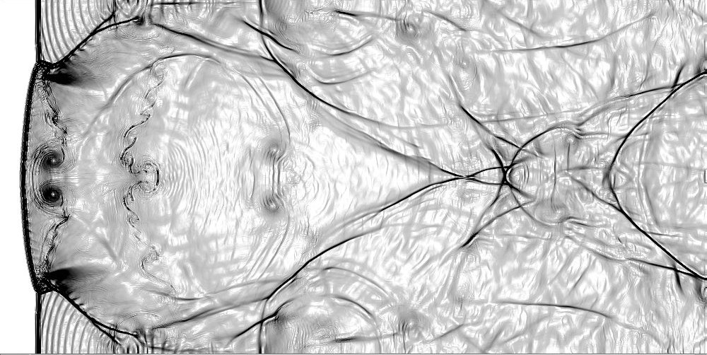
The next pictures show the pressure and temperature fields for one
time step. (JPEG, 140k each).